




In a previous article, we explored the origins of the word “statistics”, tracing it back to statecraft and the exhaustive enumeration of citizens and resources. For centuries, the golden rule of statistics was simple: to know the truth about a population, you must count every single person.
But must truth always require total enumeration? If a carefully designed sample reflects the structure of the whole, perhaps it can speak for the population as a whole.
Today, we take polls and surveys for granted. Yet the transition from exhaustive counting (a census) to drawing inference from a sample was one of the most fiercely debated paradigm shifts in the history of statistics. This is the story of how “small data” proved its power. Here, “small data” does not mean little data gathered carelessly; it means data collected through rigorous sampling design.
The Early Pioneers
Long before the mathematics of probability were formalised, a few brave thinkers tried to infer from partial data about entire populations.
The earliest notable attempt came in 1662, when the English merchant John Graunt (1620–1674) set out to estimate the population of London. Graunt was fascinated by the Bills of Mortality — weekly mortality statistics published in London. He estimated the total population of London, a figure the government did not actually know, based on the mortality rates:
- He observed from the data that there were, on average, about 13,000 deaths per year in London.
- Based on his observations, he estimated that 3 out of every 11 families experienced a death in a given year.
- Using the “Rule of Three” (basic proportions), he calculated that if 3 deaths correspond to 11 families, then 13,000 deaths correspond to approximately 47,667 families.
- He then estimated that the average household consisted of 8 people: a husband, a wife, three children, and three lodgers or servants.
- Multiplying 47,667 families by 8 people per household gave him an estimated population of roughly 381,338.
Graunt also cross-referenced his numbers using birth records:
- He observed that there were typically about 12,000 baptisms, which he equated with births, annually.
- On the assumption that women aged 16–40 had a child every other year, there must have been about 24,000 women of childbearing age contributing to those births. If they accounted for half of all women, then there were about 48,000 women in London.
- On the further assumptions that this implied roughly 48,000 households, and that the average household consisted of 8 people, the total population would be 384,000.
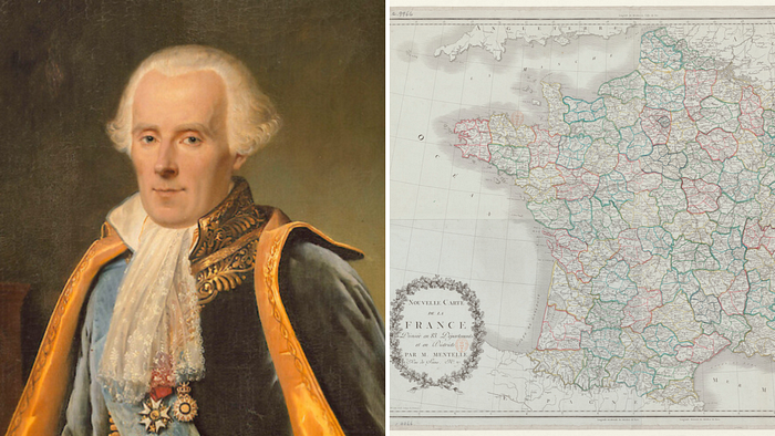
Over a century later, in 1783, the brilliant French mathematician Pierre-Simon de Laplace (1749–1827) applied a more rigorous version of this idea to estimate the population of France. At the time, conducting a full census of so large a country was prohibitively expensive and logistically impractical. Laplace proposed a clever workaround: sampling a few representative regions and calculating the ratio of inhabitants to births.
Rather than making a rough guess, Laplace asked the French government to conduct an exhaustive population count in 30 specific departments (administrative districts) spread across the country. He deliberately selected these regions to represent a diverse cross-section of French climates and topographies. In these sampled areas, the population was counted at roughly 2 million people. He then used parish registers to determine the exact number of births in those same regions over a three-year period.
By calculating the ratio of inhabitants to births in his sample and multiplying this ratio by the total number of registered births in the entire country, he could estimate the total population.
Mathematically, Laplace’s ratio estimator looked like this:

Where:
- Ŷ is the estimated total population.
- y is the population counted in the sampled regions (=2,037,615).
- x is the number of births in the sampled regions (=71,866).
- X is the total number of births in the entire country (≈1,000,000).
Using this method, Laplace estimated the population of France to be roughly 28.3 million. But his real genius lay in what he did next. Laplace used early probability theory to estimate the “error to be feared”, foreshadowing later developments that would feed into the Central Limit Theorem. He did not just provide a single number; he calculated that the odds were about 1,000 to 1 against his estimate being off by more than half a million people.
The Dogma of the Exhaustive Census
However, despite his mathematical brilliance and his pioneering effort to quantify uncertainty — what we might now recognise as an early form of interval estimation — the 19th century was dominated by the belief that statistics required exhaustive enumeration. The development of statistics was inseparable from the emergence of modern states, whose main concern was to inventory national resources. In this context, sampling was widely rejected as an inexact and fundamentally unscientific procedure.
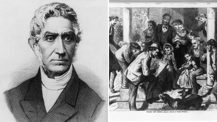
The Belgian statistician Adolphe Quételet (1796–1874), a highly influential figure in 19th-century official statistics, initially considered using Laplace’s method to estimate the population of the Netherlands in 1824 (Belgium was part of the Netherlands at that time). However, he was swayed by a severe critique from Baron de Keverberg, a Belgian statesman, who argued against partial data:
“In my opinion, there is only one way to arrive at an exact knowledge of the population and the elements of which it is composed: it is that of an actual and detailed enumeration; that is to say, the formation of nominative states of all the inhabitants, with indication of their age and occupation. Only by this mode of operation can reliable documents be obtained on the actual number of inhabitants of a country…”
Quételet subsequently became a staunch advocate of exhaustive censuses. In an 1846 letter to the Duke of Saxe-Coburg Gotha, Quételet explicitly warned against Laplace’s indirect method, arguing that accuracy was the foundational principle of statistical science:
“To not obtain the faculty of verifying the documents that are collected is to fail in one of the principal rules of science. Statistics is valuable only by its accuracy; without this essential quality, it becomes null, dangerous even, since it leads to error.”
The Danger of Naive Sampling
Why were 19th-century statisticians so afraid of partial data? Because a badly chosen sample can lead to wildly inaccurate conclusions.
Imagine a city of 100,000 people in which we want to estimate average income: 90% of residents live in middle- and low-income neighbourhoods, while 10% live in wealthy areas. If we sample 1,000 people only from the wealthiest neighbourhoods, the resulting estimate will drastically overstate the city’s average income. But if we randomly select 1,000 people from the entire population, the sample estimate will usually be much closer to the true population mean.
Without a rigorous methodology, “small data” is simply bad data. This fear kept the exhaustive census as the only accepted method for decades.
The Turning Point: Kiær’s “Representative Method”
The dogma of the exhaustive census was finally challenged in 1895 by Anders Nicolai Kiær (1838–1919), the Director of the Central Statistical Office of Norway. At the Congress of the International Statistical Institute (ISI) in Bern, Kiær presented his “representative method”.
Kiær had conducted a survey of retirement and sickness insurance schemes in Norway by selecting a sample of cities and then selecting individuals based on the first letter of their surnames. Specifically, he divided the population into cities and rural areas. Out of 61 cities, he purposively selected 13 that he regarded as “representative”. He used highly specific sampling fractions: in Oslo, he enumerated every house on 1/20 of the smallest streets; half of the houses on 1/10 of the second category of streets; and for the third category, he enumerated every fifth house on 1/4 of the streets. Enumerators were instructed to follow specific paths to ensure they captured a mix of wealthy, middle-class, and poor households. Using this representative method, he collected about 80,000 responses.
He argued that if a sample was a true “miniature” of the population, reflecting its diversity in the right proportions, it could yield highly accurate results.
Kiær’s presentation sparked a heated debate and was met with fierce hostility. Georg von Mayr (1841–1925), a German statistician and economist, forcefully opposed Kiær:
“It is especially dangerous to call for this system of representative investigations within an assembly of statisticians. It is understandable that for legislative or administrative purposes such limited enumeration may be useful — but then it must be remembered that it can never replace complete statistical observation. […] But we must remain firm and say: no calculation where observation can be done.”
Other economists like Guillaume Milliet of Switzerland echoed this sentiment, arguing that partial data was fundamentally unscientific:
“I believe that it is not right to give a congressional voice to the representative method… an importance that serious statistics will never recognise…”
Kiær, however, refused to back down, defending his method at subsequent congresses in 1897, 1901, and 1903.
The Math That Made Sampling Scientific: Arthur Bowley and the Central Limit Theorem
Kiær had the right instinct. He understood that, if chosen with care, a small part of the population could reveal something meaningful about the whole. Yet he was unable to answer the question that mattered most: why should anyone trust the result?
Because Kiær selected his samples by human judgement (what we would now call purposive or non-probability sampling), there was no objective way to measure how precise his estimates really were. If a critic asked, “How far might your estimate be from the truth?” he had little to offer beyond his own care, experience, and conviction.
That began to change with the British statistician Arthur Bowley (1869–1957). Bowley helped place sampling on firmer mathematical ground. His crucial insight was simple but profound: the key to measuring error was not judgement, but randomness. Once every unit in a population (e.g. a person, a household, a company) had a known chance of being selected, uncertainty no longer had to be guessed at. It could be calculated and analysed.
In 1906, Bowley showed how the Central Limit Theorem could be brought to bear on sampling from finite populations. In essence, the theorem says this: even when the original population is irregular or strongly skewed, the means of sufficiently large random samples will tend to follow an approximately normal (bell-shaped) distribution.
In simplified form, if a population has mean μ and variance σ², then the sample mean ȳ from a random sample of size n is approximately distributed as:

This was a turning point. It showed that sampling error grows smaller as sample size grows larger, and it gave statisticians a theoretically-sound way to quantify uncertainty. From this flowed the modern language of margins of error and confidence intervals. In other words, a well-drawn small sample could speak for a much larger population, and do so with measurable limits of uncertainty.
(The animation below shows how repeated sample means gradually form a bell-shaped distribution, even when the true population distribution is highly skewed, like the income distribution above.)
Bowley did not stop with simple random sampling. He recognised that chance alone, though essential, could sometimes be unkind. A random sample might, purely by accident, include too many people from one group and too few from another.
His answer was stratified sampling. Rather than drawing from the population in a single sweep, Bowley proposed dividing it into more homogeneous groups called “strata”, such as regions, age groups, or income bands, and then drawing a random sample from each stratum in proportion to its size in the population.
The intuition is straightforward: when the important subgroups of a population are represented in the right proportions, estimates tend to become steadier and more precise. Bowley showed mathematically that, when strata do not overlap, units are sampled randomly within each stratum, and the sample is allocated in proportion to stratum size, the sampling variance of a stratified estimator is less than or equal to that of a simple random sample of the same total size.